Quickstart with Syncopy#
Here we want to quickly explore some standard analyses for analog data (e.g. MUA or LFP measurements), and how to do these in Syncopy. Explorative coding is best done interactively by using e.g. Jupyter or IPython. Note that for plotting also matplotlib has to be installed.
Users coming from FieldTrip should also have a look at the Syncopy for FieldTrip Users section.
Note
Installation of Syncopy itself is covered in here.
Preparations#
To start with a clean slate, let’s construct a synthetic dataset consisting of a damped 30Hz harmonic and additive red noise acting as a 1/f surrogate:
import numpy as np
import syncopy as spy

# cfg dictionary
cfg = spy.StructDict()
cfg.nTrials = 50
cfg.nSamples = 1000
cfg.nChannels = 2
cfg.samplerate = 500   # in Hz

# 30Hz undamped harmonic
harm = spy.synthdata.harmonic(cfg, freq=30)

# red noise with seed for exact reproducibility
noise = spy.synthdata.red_noise(cfg, alpha=0.9, seed=42)
To look at a single trial we can use the .trials property of Syncopy data objects, which behaves similar to Python lists where each element is a trial represented as a numpy.ndarray:
# how many trials do we have?
print(harm.trials)
>>> 50 element iterable

# access the 1st trial as numpy array
print(harm.trials[0].shape)
>>> (1000, 2)

# show order of dimensions
print(harm.dimord)
>>> ['time', 'channel']
So we see that as defined above we indeed have 50 trials, with each having 1000 samples and 2 channels.
For now we have two distinct datasets harm and noise, we can combine them using standard arithmetic Python operators. But first let’s actually dampen the harmonic and zero out the 2nd channel:
# pseudo 2d array with shape (1000, 1) for the dampening
harm = harm * np.linspace(1, 0.2, cfg.nSamples)[:, np.newaxis]

# zero out 2nd channel with a (2,) shaped array
harm = harm * np.array([1, 0])
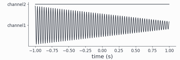
To check that we got a damped harmonic on the first and just zeros on the second channel we can plot an arbitrary trial:
# plot the 20th trial
harm.singlepanelplot(trials=19)
Finally we can just add our red noise dataset to arrive at our final synthetic dataset:
# scale the noise up a bit
adata = harm + 1.2 * noise

# rename the channels
adata.channel = ['30Hz + noise', 'noise only']
Note
Syncopy arithmetics follow NumPy’s broadcasting rules on a trial-by-trial basis. Meaning single arrays which are broadcastable to every trial OR Syncopy datasets where each trial-pair of both datasets is shape compatible are valid operands.
adata is a dataset of type AnalogData, which is intended for holding time-series data like electrophysiological measurements. Let’s have a look at a small snippet of the first trial:
adata.singlepanelplot(trials=0, latency=[0, 0.5])
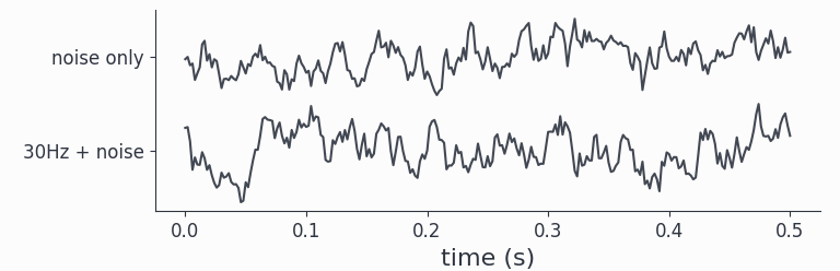
By construction, we made the red noise of similar strength as the signal, hence by eye the oscillations present in channel1 are hardly visible. The parameter latency defines a time-interval selection.
Note
How to plot and work with subsets of Syncopy data is described in Selections.
To recap: we have generated a synthetic dataset whith red noise on both channels, and channel1 additionally carries the damped harmonic signal.
Note
Further details about artificial data generation can be found at the Synthetic Data section.
Data Object Inspection#
We can get some basic information about any Syncopy dataset by just typing its name in an interactive Python interpreter:
adata
which gives nicely formatted output:
Syncopy AnalogData object with fields

         cfg : dictionary with keys ''
     channel : [2] element <class 'numpy.ndarray'>
   container : None
        data : 50 trials of length 1000.0 defined on [50000 x 2] float64 Dataset of size 0.76 MB
      dimord : time by channel
    filename : /xxx/xxx/.spy/spy_910e_572582c9.analog
        mode : r+
  sampleinfo : [50 x 2] element <class 'numpy.ndarray'>
  samplerate : 500.0
         tag : None
        time : 50 element list
   trialinfo : [50 x 0] element <class 'numpy.ndarray'>
      trials : 50 element iterable

Use `.log` to see object history
So we see that we indeed got 50 trials with 2 channels and 1000 samples each. Note that Syncopy per default stores and writes all data on disk, as this allows for seamless processing of larger than memory datasets. The exact location and filename of a dataset in question is listed at the filename field. The standard location is the .spy directory created automatically in the user’s home directory. To change this and for more details please see Setting Up Your Python Environment.
Hint
You can access each of the shown meta-information fields separately using standard Python attribute access, e.g. data.filename or data.samplerate.
Spectral Analysis#
Syncopy groups analysis functionality into meta-functions, which in turn have various parameters selecting and controlling specific methods. In the case of spectral analysis the function to use is freqanalysis().
Here we quickly want to showcase two important methods for (time-)frequency analysis: (multi-tapered) FFT and Wavelet analysis.
Multitapered Fourier Analysis#
Multitaper methods allow for frequency smoothing of Fourier spectra. Syncopy implements the standard Slepian/DPSS tapers and provides a convenient parameter, the taper smoothing frequency tapsmofrq to control the amount of one-sided spectral smoothing in Hz. To perform a multi-tapered Fourier analysis with 2Hz spectral smoothing (1Hz two sided), we simply do:
# increase log level
spy.set_loglevel("INFO")

# compute the spectra
fft_spectra = spy.freqanalysis(adata, method='mtmfft', foilim=[0, 60], tapsmofrq=1)
The parameter foilim controls the frequencies of interest limits, so in this case we are interested in the range 0-60Hz. Starting the computation interactively will show additional information:
Syncopy <validate_taper> INFO: Using 3 taper(s) for multi-tapering
informing us, that for this dataset a total spectral smoothing of 2Hz required 3 Slepian tapers.
The resulting new dataset fft_spectra is of type syncopy.SpectralData, which is the general datatype storing the results of a time-frequency analysis.
Hint
Try typing fft_spectra.log into your interpreter and have a look at Trace Your Steps: Data Logs to learn more about Syncopy’s logging features
To quickly have something for the eye we can compute the trial average and plot the power spectrum using the generic syncopy.singlepanelplot():
# compute trial average
fft_avg = spy.mean(fft_spectra, dim='trials')

# plot frequency range between 10Hz and 50Hz
fft_avg.singlepanelplot(frequency=[2, 60])
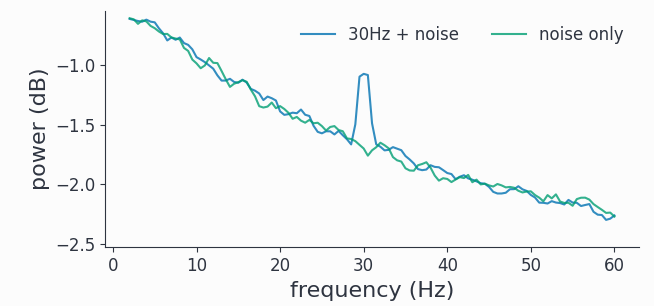
We clearly see a smoothed spectral peak at 30Hz, channel 2 just contains the red noise with its 1/f characteristic. Comparing with the signals plotted in the time domain above, we see the benefit of the frequency representation of an oscillatory signal.
The related short time Fourier transform can be computed via method='mtmconvol', see freqanalysis() for more details and examples.
Note
Have a look at this section to get an overview about data processing principles with Syncopy
Note
Have a look at Syncopy Data Classes to get an overview over the different data types of Syncopy
Wavelet Analysis#
Wavelet Analysis, especially with Morlet Wavelets, is a well established method for time-frequency analysis. For each frequency of interest (foi), a Wavelet function gets convolved with the signal yielding a time dependent cross-correlation. By (densely) scanning a range of frequencies, a continuous time-frequency representation of the original signal can be generated.
In Syncopy we can compute the Wavelet transform by calling freqanalysis() with the method='wavelet' argument:
# define frequencies to scan
fois = np.arange(10, 50, step=0.5) # 0.5Hz stepping
wav_spectra = spy.freqanalysis(adata,
                               method='wavelet',
                               foi=fois,
                               keeptrials=False)
Here we used an additional parameter supported by every Syncopy analysis method:
keeptrials=Falsetrial averaging of the result
Hint
Have a look at the Parallel Processing section for information about concurrent computations with Syncopy.
To quickly inspect the results for each channel we can use:
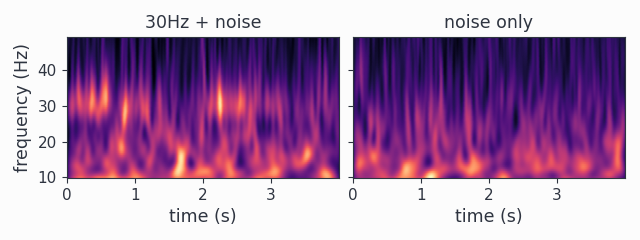
wav_spectra.multipanelplot()
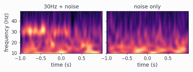
Again, we see a 30Hz signal in the 1st channel, and channel 2 is dominated by aperiodic dynamics resembling 1/f. However, in contrast to the method='mtmfft' call, now we also get information along the time axis. The dampening of the 30Hz harmonic over time in the first channel is clearly visible.
An improved method, the superlet transform, providing super-resolution time-frequency representations can be computed via method='superlet', see freqanalysis() for more details.
Trialdefinition#
The .trialdefinition property controls how individual trials are defined from the underlying continuous data array. Let’s have a look at the default trial definition coming from the synthetic data routines:
adata.trialdefinition
This gives an output:
array([[    0.,  1000.,  -500.],
     [ 1000.,  2000.,  -500.],
     [ 2000.,  3000.,  -500.],
     ...
     ]])
We see it is a nSamples x 3 numpy.ndarray, encoding [start, stop, offset] for each trial. Using NumPy we can create a new trialdefinition:
# create simple trialdefinition array
trl_def = np.array([[i * 2000, (i + 1) * 2000, 0] for i in range(25)])

# copy original dataset
adata2 = adata.copy()
adata2.trialdefinition = trl_def
Here we effectively concatenated all consecutive trials, with the new trials being each 2000 samples long. If we inspect adata2 now:
adata2.trials
>>> 25 element iterable
we see that now we only have 25 trials. And the trialdefinition looks accordingly:
adata2.trialdefinition
>>> array([[    0,  2000,     0],
     [ 2000,  4000,     0],
     [ 4000,  6000,     0],
     ...]])
Warning
Data which is not covered by the trial definition gets stripped off the dataset after each and every operation (including selections!) to save disc space. Hence copying before applying a new trialdefinition is highly recommended.
Repeating the wavelet analysis reusing the fois defined above:
wav_spectra2 = spy.freqanalysis(adata2,
                                method='wavelet',
                                foi=fois,
                                keeptrials=False)

wav_spectra2.multipanelplot()
We now see the trials are 4 seconds long (2000 samples times 1/500Hz = 4s), so the time axis automatically changed according to the new trialdefinition. Also the trials now start at zero seconds, as we set the offsets to zero. As we have now chained two damped harmonics together, we can see 30Hz epochs in the first channel.