Running Welch’s method for the estimation of power spectra in Syncopy#
Welch’s method for the estimation of power spectra based on time-averaging over short, modified periodograms is described in the following publication (DOI link):
Welch, P. (1967). The use of fast Fourier transform for the estimation of power spectra: a method based on time averaging over short, modified periodograms. IEEE Transactions on Audio and Electroacoustics, 15(2), 70-73.
In short, it splits the original time-domain signal into several, potentially overlapping, segments. A taper (window function) is then applied on each segment individually, and each segment is transferred into the frequency domain by computing the FFT. Computing the squared magnitude results in one periodogram per segment. Welch refers to these as modified periodograms in the publication, because of the taper that has been applied. These powers are averaged over the windows to obtain the final estimate of the power spectrum.
Due to the averaging, Welch’s method works well with noisy data: the averaging reduces the variance of the estimator. The price to pay is a reduced frequency resolution due to the short input segments compared to the single, full-sized signal.
Generating Example Data#
Let us first prepare suitable data, we use white noise here:
1import syncopy as spy
2from syncopy import synthdata
3
4wn = synthdata.white_noise(nTrials=2, nChannels=3, nSamples=20000, samplerate=1000)
The return value wn is of type AnalogData and contains 2 trials and 3 channels,
each consisting of 20 seconds of white noise: 20000 samples at a sample rate of 1000 Hz. We can show this easily:
1wn.dimord       # ['time', 'channel']
2wn.data.shape   # (40000, 3)
3wn.trialdefinition # array([[    0., 20000., -1000.], [20000., 40000., -1000.]])
Spectral Analysis using Welch’s Method#
We now create a config for running Welch’s method and call freqanalysis with it:
1cfg = spy.StructDict()
2cfg.method = "welch"
3cfg.t_ftimwin = 0.5  # Window length in seconds.
4cfg.toi = 0.5        # Overlap between windows, 0.5 = 50 percent overlap.
5
6welch_psd = spy.freqanalysis(cfg, wn)
Let’s inspect the resulting SpectralData instance by looking at its dimensions, and then visualize it:
1welch_psd.dimord      # ('time', 'taper', 'freq', 'channel',)
2welch_psd.data.shape  # (2, 1, 251, 3)
The shape is as expected:
The time axis contains two entries, one per trial, because by default there is no trial averaging (keeptrials is True). With trial averaging, there would only be a single entry here.
The taper axis will always have size 1 for Welch, even for multi-tapering, as tapers must be averaged for Welch’s method (keeptapers must be False), as explained in the function documentation.
The size of the frequency axis (freq, 251 here), i.e., the frequency resolution, depends on the signal length of the input windows and is thus a function of the input signal, t_ftimwin and toi, and potentially other settings (like a foilim, i.e. limiting the frequencies of interest).
The channels are unchanged, as we receive one result per channel.
We can also visualize the power spectrum. Here we select the first of the two trials:
1_, ax = welch_psd.singlepanelplot(trials=0, logscale=False)
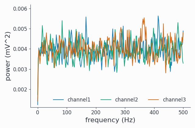
We can see the estimated power flat spectrum for three channels of white noise.
Note
If you run the lines above in your Python interpreter but no plot window opens, you may need to first configure matplotlib for interactive plotting like this: `import matplotlib.pyplot as plt; plt.ion()`. Then re-run the plotting commmands.
Available Settings#
Many settings affect the outcome of a Welch run, including:
t_ftimwin : window length (a.k.a. segment length) in seconds.
toi : overlap between windows, 0.5 = 50 percent overlap.
foilim : frequencies of interest, a specific frequency range, e.g. set to
[5, 100]to get results between 5 to 100 Hz.taper and tapsmofrq : for taper selection and multi-tapering. Note that in case of multi-tapering, the data in the windows will be averaged across the tapers first
keeptrials : whether trials should be left as-is, or you want a trial-average. If
False, and thus trial-averaging is requested, it will happen on the raw data in the time domain, before Welch is run.
Comparison with raw FFT#
Let’s compare Welch’s result with the raw FFT estimate:
fft_psd = spy.freqanalysis(wn)
fft_psd.singlepanelplot(trials=0, channel=0, logscale=False)
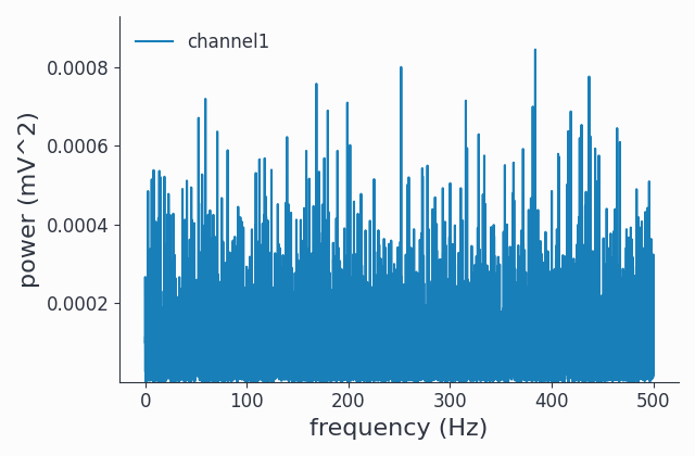
The power spectral esimtate is much more noisy, meaning the variance per frequency bin is considerably larger compared to Welch’s estimate.
Note
We don’t need any parameters for freqanalysis here, as method='mtmfft' and tapsmofrq=None are the defaults.
Note that the absolute power values are lower, as we have a lot more frequency bins when calculating the raw FFT at once for the unsegmented signal:
fft_psd.freq.shape   # (10001,)
welch_psd.freq.shape   # (251,)
Syncopy normalizes spectral power per 1Hz bin, meaning that the noise power gets diluted over many more frequency bins when using the raw FFT. We can check that by summing over the frequency axis for both estimates:
np.sum(fft_psd.show(trials=0, channel=0))   # will be ~1
np.sum(welch_psd.show(trials=0, channel=0))   # will also be ~1
Investigating the Effects of the Overlap Parameter as a Function of Signal Length#
Here, we want to illustrate the effects of the chosen overlap between windows (toi), on signals of different lengths.
For this, we investigate various combinations of signal length and overlap. For each combination, we realize several instantiations of white noise and run Welch’s method to get an estimate of the power spectral density. We then compute the variance of the estimates. Here is a visualization of the result (source):
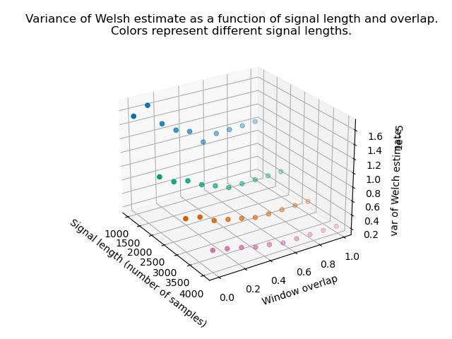
From this plot we can conclude several things. First, as expected, with all settings fixed, a longer signal (and thus an increased number of segments) reduces the variance of the estimate. Second, up to a certain level (somewhere around 0.5 to 0.6), increasing the overlap also reduces the variance of the estimator. However, if you go too high, the variance starts increasing again. The whole effect is most pronounced for short signals, but these are the typical case in neuroscience.
The plot suggests that it may be helpful to try an overlap of around 0.5 for short signals, by setting `cfg.toi=0.5`.
This concludes the tutorial on using Welch’s method in Syncopy.