Connectivity Analysis#
Having time-frequency results for individual channels is useful, however we hardly learn anything about functional relationships between different sources. Even if two channels have a spectral peak at say 100Hz, we don’t know if these signals are actually connected. Syncopy offers various distinct methods to elucidate such putative connections via the connectivityanalysis() meta-function: coherence, cross-correlation and Granger-Geweke causality.
AR(2) Models#
To have a synthetic albeit meaningful dataset to illustrate the different methodologies we start by simulating three autoregressive processes of order 2:
import numpy as np
import syncopy as spy
from syncopy import synthdata

cfg = spy.StructDict()
cfg.nTrials = 50
cfg.nSamples = 2000
cfg.samplerate = 250

# 3x3 Adjacency matrix to define coupling
AdjMat = np.zeros((3, 3))
# only coupling 0 -> 1
AdjMat[0, 1] = 0.2

data = synthdata.ar2_network(AdjMat, cfg=cfg, seed=42)

# add some red noise as 1/f surrogate
data = data + 2 * synthdata.red_noise(cfg, alpha=0.95, nChannels=3, seed=42)

spec = spy.freqanalysis(data, tapsmofrq=3, keeptrials=False)
We also right away calculated the respective power spectra spec.
We can quickly have a look at a snippet of the generated signals:
data.singlepanelplot(trials=0, latency=[0, 1.])
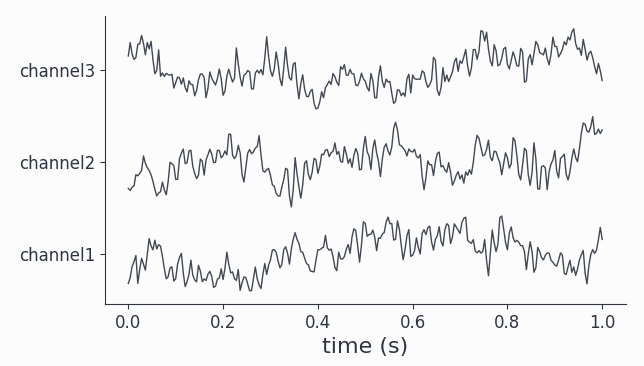
All channels show visible oscillations as is confirmed by looking at the power spectra:
spec.singlepanelplot()
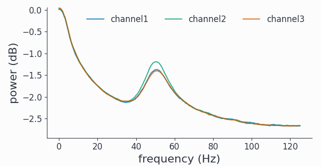
As expected for the stochastic AR(2) model, we have a fairly broad spectral peak at around 50Hz plus the 1/f like background.
Coherence#
One way to check for relationships between different oscillating channels is to calculate the pairwise coherence measure. It can be roughly understood as a frequency dependent correlation. Let’s do this for our coupled AR(2) signals:
coherence = spy.connectivityanalysis(data, method='coh', tapsmofrq=3)
The result is of type CrossSpectralData, the standard datatype for all connectivity measures. It contains the results for all nChannels x nChannels possible combinations. Let’s pick a few available channel combinations and plot the results:
coherence.singlepanelplot(channel_i='channel1', channel_j='channel2')
coherence.singlepanelplot(channel_i='channel2', channel_j='channel1')
coherence.singlepanelplot(channel_i='channel3', channel_j='channel1')
coherence.singlepanelplot(channel_i='channel3', channel_j='channel2')
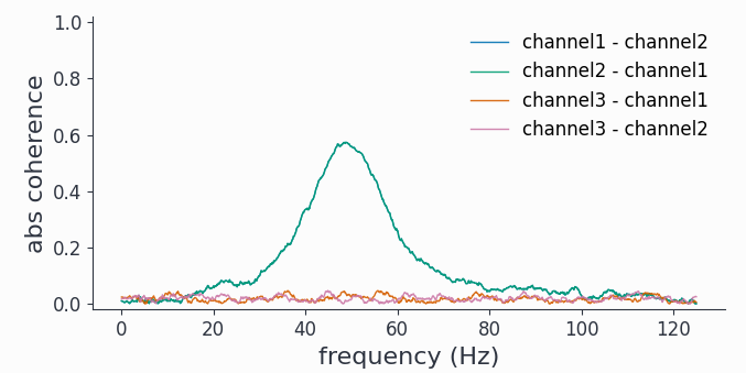
As coherence is a symmetric measure, we obtain exactly the same graph for both channel1-channel2 combinations, showing high coherence around 50Hz. However as channel3 is completely uncoupled, there is no coherence with either channel1 or channel2.
Note
The plotting for CrossSpectralData objects works a bit differently, as the user here has to provide one channel combination for each plot with the keywords channel_i and channel_j.
Cross-Correlation#
Coherence is a spectral measure for correlation, the corresponding time-domain measure is the well known cross-correlation. In Syncopy we can get the cross-correlation between all channel pairs with:
corr = spy.connectivityanalysis(data, method='corr', keeptrials=True)
As this also is a symmetric measure, we just look at only one channel combination for each channel pair:
corr.singlepanelplot(channel_i=0, channel_j=1, trials=1)
corr.singlepanelplot(channel_i=0, channel_j=2, trials=1)
corr.singlepanelplot(channel_i=1, channel_j=2, trials=1)
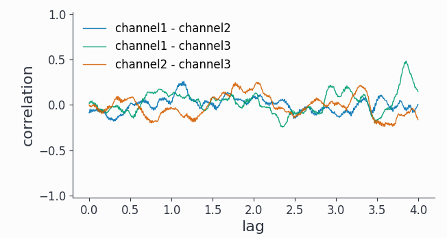
As a time domain measure, the cross-correlation is confounded by the 1/f background present in all 3 channels.
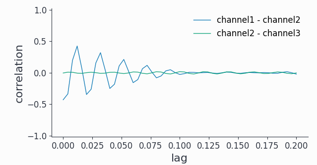
We can however use a bandpass filter around 50Hz first and then trial average the cross-correlations to unmask some short-lived (~0.1s) correlations between channel1 and channel2:
bp_filtered = spy.preprocessing(data, filter_type='bp', freq=[45, 55])
bp_corr = spy.connectivityanalysis(bp_filtered, method='corr', keeptrials=False)

# look only at lags of max. 0.2 seconds
bp_corr.singlepanelplot(channel_i=0, channel_j=1, latency=[0, 0.2])
bp_corr.singlepanelplot(channel_i=1, channel_j=2, latency=[0, 0.2])
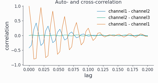
Note that we can also look at the auto-correlation:
fig, ax =  bp_corr.singlepanelplot(channel_i=0,
                                   channel_j=0,
                                   latency=[0, 0.2])

ax.set_title('Auto- and cross-correlation')
Hint
Have a look at the Preprocessing section to learn more about pre-processing data with Syncopy.
Granger Causality#
To reveal directionality, or causality, between different channels Syncopy offers the Granger-Geweke algorithm for non-parametric Granger causality in the spectral domain:
granger = spy.connectivityanalysis(data, method='granger', tapsmofrq=2)
Now we want to see differential causality, so we plot more channel combinations:
granger.singlepanelplot(channel_i=0, channel_j=1)
granger.singlepanelplot(channel_i=1, channel_j=0)
granger.singlepanelplot(channel_i=0, channel_j=2)
fig, ax = granger.singlepanelplot(channel_i=2, channel_j=0)
ax.set_ylim((-.05, 0.6))
This reveals the coupling structure we put into this synthetic data set: channel1 influences channel2, but in the other direction there is no interaction. The oscillations in channel3 are completely uncoupled.
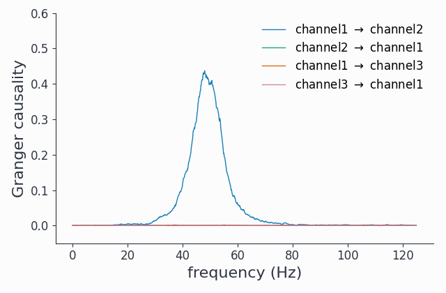
As a spectral method, we did not need to filter out any 1/f component to uncover the coupling topology.
Note
The keeptrials keyword is only valid for cross-correlations, as both Granger causality and coherence critically rely on trial averaging.