Synthetic Data

For testing and educational purposes it is always good to work with synthetic data. Syncopy brings its own suite of synthetic data generators, but it is also possible to devise your own synthetic data using standard NumPy.

Built-in Generators

These functions return a multi-trial AnalogData object representing multi-channel time series data:

syncopy.synthdata.harmonic(freq, samplerate)	A harmonic with frequency freq.
syncopy.synthdata.white_noise([nSamples, ...])	Plain white noise with unity standard deviation.
syncopy.synthdata.red_noise(alpha[, ...])	Uncoupled multi-channel AR(1) process realizations.
syncopy.synthdata.linear_trend(y_max[, ...])	A linear trend on all channels from 0 to y_max in nSamples.
syncopy.synthdata.phase_diffusion(freq[, ...])	Linear (harmonic) phase evolution plus a Brownian noise term inducing phase diffusion around the deterministic phase velocity (angular frequency).
syncopy.synthdata.ar2_network([AdjMat, ...])	Simulation of a network of coupled AR(2) processes

With the help of basic arithmetical operations we can combine different synthetic signals to arrive at more complex ones. Let’s look at an example:

import syncopy as spy

# set up cfg
cfg = spy.StructDict()
cfg.nTrials = 40
cfg.samplerate = 500
cfg.nSamples = 500
cfg.nChannels = 5

# start with a simple 60Hz harmonic
sdata = spy.synthdata.harmonic(freq=60, cfg=cfg)

# add some strong AR(1) process as surrogate 1/f
sdata = sdata + 5 * spy.synthdata.red_noise(alpha=0.95, cfg=cfg)

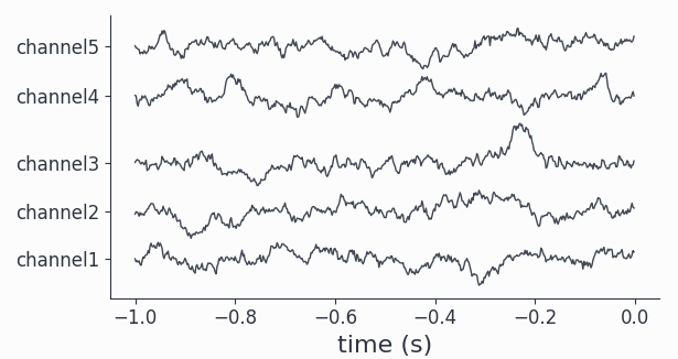
# plot all channels for a single trial
sdata.singlepanelplot(trials=10)

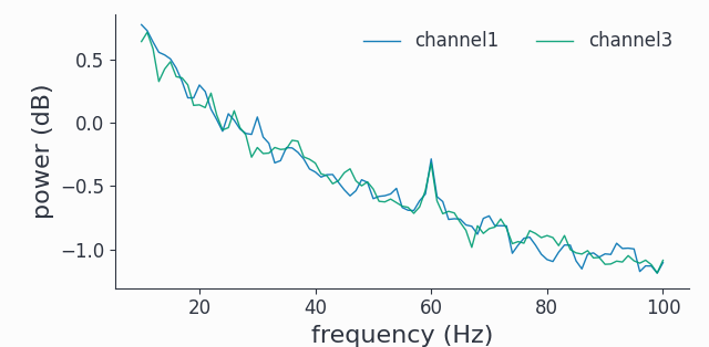
# compute spectrum and plot trial average of 2 channels
spec = spy.freqanalysis(sdata, keeptrials=False)
spec.singlepanelplot(channel=[0, 2], frequency=[0,100])

Phase diffusion

A diffusing phase can be modeled by adding white noise \(\xi(t)\) to a fixed angular frequency:

\[\omega(t) = \omega + \epsilon \xi(t),\]

with the instantaneous frequency \(\omega(t)\).

Integration then yields the phase trajectory:

\[\phi(t) = \int_0^t \omega(t) = \omega t + \epsilon W(t).\]

Here \(W(t)\) being the Wiener process, or simply a one dimensional diffusion process. Note that for the trivial case \(\epsilon = 0\), so no noise got added, the phase describes a linear constant motion with the phase velocity \(\omega = 2\pi f\). This is just a harmonic oscillation with frequency \(f\). Finally, by wrapping the phase trajectory into a \(2\pi\) periodic waveform function, we arrive at a time series (or signal). The simplest waveform is just the cosine, so we have:

\[x(t) = cos(\phi(t))\]

This is exactly what the phase_diffusion() function provides.

Phase diffusing models have some interesting properties, let’s have a look at the power spectrum:

import syncopy as spy

cfg = spy.StructDict()
cfg.nTrials = 250
cfg.nChannels = 2
cfg.samplerate = 500
cfg.nSamples = 2000

# harmonic frequency is 60Hz, phase diffusion strength is 0.01
signals = spy.synthdata.phase_diffusion(freq=60, eps=0.01, cfg=cfg)

# add harmonic frequency with 20Hz, there is no phase diffusion
signals += spy.synthdata.harmonic(freq=20, cfg=cfg)

# freqanalysis without tapering and absolute power

cfg_freq = spy.StructDict()
cfg_freq.keeptrials = False
cfg_freq.foilim = [2, 100]
cfg_freq.output = 'abs'
cfg_freq.taper = None

spec = spy.freqanalysis(signals, cfg=cfg_freq)
spec.singlepanelplot(channel=0)

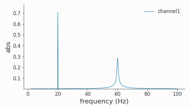
We see a natural (no tapering) spectral broadening for the phase diffusing signal at 60Hz, reflecting the fluctuations in instantaneous frequency.

General Recipe for custom Synthetic Data

We can easily create custom synthetic datasets using basic NumPy functionality and Syncopy’s AnalogData.

To create a synthetic timeseries data set follow these steps:

• write a function which returns a single trial as a 2d-ndarray with desired shape (nSamples, nChannels)

• collect all the trials into a Python list, for example with a list comprehension or simply a for loop

• Instantiate an AnalogData object by passing this list holding the trials as data and set the desired samplerate

In (pseudo-)Python code:

def generate_trial(nSamples, nChannels):

     trial = .. something fancy ..

     # These should evaluate to True
     isinstance(trial, np.ndarray)
     trial.shape == (nSamples, nChannels)

     return trial

# collect the trials
nSamples = 1000
nChannels = 2
nTrials = 100
trls = []

for _ in range(nTrials):
    trial = generate_trial(Samples, nChannels)
    # manipulate further as needed, e.g. add a constant
    trial += 3
    trls.append(trial)

# instantiate syncopy data object
my_fancy_data = spy.AnalogData(data=trls, samplerate=my_samplerate)

Note

The same recipe can be used to generally instantiate Syncopy data objects from NumPy arrays.

Note

Syncopy data objects also accept Python generators as data, allowing to stream in trial arrays one by one. In effect this allows creating datasets which are larger than the systems memory. This is also how the build in generators of syncopy.synthdata (see above) work under the hood.

Example: Noisy Harmonics

Let’s create two harmonics and add some white noise to it:

import numpy as np
import syncopy as spy


def generate_noisy_harmonics(nSamples, nChannels, samplerate):

    f1, f2 = 20, 50 # the harmonic frequencies in Hz

    # the sampling times vector
    tvec = np.arange(nSamples) * 1 / samplerate

    # define the two harmonics
    ch1 = np.cos(2 * np.pi * f1 * tvec)
    ch2 = np.cos(2 * np.pi * f2 * tvec)

    # concatenate channels to to trial array
    trial = np.column_stack([ch1, ch2])

    # add some white noise
    trial += 0.5 * np.random.randn(nSamples, nChannels)

    return trial


nTrials = 50
nSamples = 1000
nChannels = 2
samplerate = 500   # in Hz

# collect trials
trials = []
for _ in range(nTrials):
    trial = generate_noisy_harmonics(nSamples, nChannels, samplerate)
    trials.append(trial)

synth_data = spy.AnalogData(trials, samplerate=samplerate)

Here we first defined the number of trials (nTrials) and then the number of samples (nSamples) and channels (nChannels) per trial. With a sampling rate of 500Hz and 1000 samples this gives us a trial length of two seconds. The function generate_noisy_harmonics adds a 20Hz harmonic on the 1st channel, a 50Hz harmonic on the 2nd channel and white noise to all channels, Every trial got collected into a Python list, which at the last line was used to initialize our AnalogData object synth_data. Note that data instantiated that way always has a default trigger offset of -1 seconds.

Now we can directly run a multi-tapered FFT analysis and plot the power spectra of all 2 channels:

spectrum = spy.freqanalysis(synth_data, foilim=[0,80], tapsmofrq=2, keeptrials=False)
spectrum.singlepanelplot()

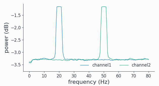
As constructed, we have two harmonic peaks at the respective frequencies (20Hz and 50Hz) and the white noise floor on all channels.