Selections

Basically every practical data analysis project involves working on subsets of the data. Syncopy offers the powerful selectdata() function to achieve exactly that. There are two distinct ways to apply a selection, either in-place or the chosen subset gets copied and returned as a new Syncopy data object. Additionally, every Syncopy meta-function (see Syncopy Meta-Functions) supports the select keyword, which applies an in place selection on the fly when processing data.

Selections are an important concept of Syncopy and are being re-used under the hood for plotting functions like singlepanelplot() and also for show(). Both plotting and numpy array extraction naturally operate on subsets of the data, and conveniently use the same selection criteria syntax as selectdata().

Creating Selections

Syncopy data objects can be best understood as n-dimensional arrays or matrices, with each dimension holding a certain property of the data. For an AnalogData object these dimensions would be time, channel and trials. Now we can define sub-slices of the data by combining index sets for each of those axes.

A new selection can be created by calling selectdata(), here we want to select a single trial and two channels:

trial10 = AData.selectdata(trials=10, channel=["channel11", "channel17"])
# alternatively
trial10 = spy.selectdata(AData, trials=10, channel=["channel02", "channel06"])

AData is an AnalogData object, and hence the resulting trial10 data object will also be of that same data type. Inspecting the original dataset by simply typing its name into the Python interpreter:

AData

we see that we have 100 trials and 10 channels:

Syncopy AnalogData object with fields

         cfg : dictionary with keys ''
     channel : [10] element <class 'numpy.ndarray'>
   container : None
        data : 100 trials of length 500.0 defined on [50000 x 10] float32 Dataset of size 1.91 MB
    ...

If we now inspect our selection results:

trial10

we see that we are left with 1 trial and 2 channels:

Syncopy AnalogData object with fields

         cfg : dictionary with keys ''
     channel : [2] element <class 'numpy.ndarray'>
   container : None
        data : 1 trials of length 500.0 defined on [500 x 2] float32 Dataset of size 0.00 MB
    ...

As we did not specify any selection criteria for the time axis (via latency) every sample was selected. This is true in general: whenever a certain dimension has no selection specification the complete axis is selected.

Finally by inspecting the .log (see also Trace Your Steps: Data Logs) we can see the selection settings used to create this dataset:

trials10.log

write_log: computed _selectdata with settings
inplace = False
clear = False
latency=None
trials = 10
channel = ['channel02', 'channel06']

This log is persistent, meaning that when saving and later loading this reduced dataset the settings used for this selection can still be recovered. The table below summarizes all possible selection parameters and their availability for each datatype.

Table of Selection Parameters

There are various selection parameters available, which each can accept a variety of Python datatypes like int, str or list. Some selection parameters are only available for data types which have the corresponding dimension, like frequency for SpectralData and CrossSpectralData.

Parameter	Description	Accepted Types	Examples	Availability
trials	trial selection	int, array, list	selectdata(trials=7) selectdata(trials=[2, 9, 21]) selectdata(trials=np.arange(2, 10))	all data types
channel	channel selection	int, str, list, array	selectdata(channel=7) selectdata(channel=[11, 16]) selectdata(channel=np.arange(2, 10)) selectdata(channel=["V1-11, "V2-12"])	AnalogData SpectralData CrossSpectralData SpikeData
latency	time interval of interest in seconds	list, float, ‘maxperiod’, ‘minperiod’, ‘prestim’, ‘poststim’	selectdata(latency=[0.2, 1.]) selectdata(latency=0.5) selectdata(latency='minperiod')	AnalogData SpectralData CrossSpectralData SpikeData
frequency	frequencies of interest in Hz	float, list	selectdata(frequency=20.5) selectdata(frequency=[5, 10, 15])	SpectralData CrossSpectralData
unit	unit selection	int, str, list, array	selectdata(unit=7) selectdata(unit=[11, 16, 32]) selectdata(unit=["unit17", "unit3"])	SpikeData
eventid	eventid selection	int, list, array	selectdata(eventid=2) selectdata(eventid=[2, 0, 1])	EventData

Note

Have a look at Data Basics for further details about Syncopy’s data classes and interfaces

Inplace Selections

An in-place selection can be understood as a mask being put onto the data. Meaning that the selected subset of the data is actually not copied on disc, but the selection criteria are applied in place to be used in a processing step. Inplace selections take two forms: either explicit via the inplace keyword selectdata(..., inplace=True), or implicit by passing a select keyword to a Syncopy meta-function.

To illustrate this mechanic, let’s create a simulated dataset with phase_diffusion() and compute the coherence for the full dataset:

import numpy as np
import syncopy as spy
from syncopy.tests import synth_data

# 100 trials of two phase diffusing signals with 40Hz
adata = synth_data.phase_diffusion(nTrials=100,
                                   freq=40,
                                   samplerate=200,
                                   nSamples=500,
                                   nChannels=2,
                                   eps=0.01)

# coherence for full dataset
coh1 = spy.connectivityanalysis(adata, method='coh')

# plot coherence of channel1 vs channel2
coh1.singlepanelplot(channel_i='channel1', channel_j='channel2')

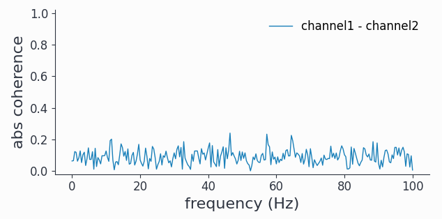
Phase diffusing signals decorrelate over time, hence if we wait long enough we can’t see any coherence.

Note

As an exercise you could use freqanalysis() to confirm that there is indeed strong oscillatory activity in the 40Hz band

Explicit inplace Selection

To see if maybe for a shorter time period in the beginning of “the recording” the signals were actually more phase locked, we can use an in-place latency selection:

# note there is no return value here
spy.selectdata(adata, latency=[-1, 0], inplace=True)

Inspecting the dataset:

Syncopy AnalogData object with fields

            cfg : dictionary with keys 'selectdata'
        channel : [2] element <class 'numpy.ndarray'>
      container : None
           data : 100 trials defined on [50000 x 3] float64 Dataset of size 1.14 MB
         dimord : time by channel
       filename : /home/whir/.spy/spy_3e83_a9c8b544.analog
           info : dictionary with keys ''
           mode : r+
     sampleinfo : [100 x 2] element <class 'numpy.ndarray'>
     samplerate : 200.0
      selection : Syncopy AnalogData selector with all channels, 201 times, 100 trials
            tag : None
           time : 100 element list
      trialinfo : [100 x 0] element <class 'numpy.ndarray'>
 trialintervals : [100 x 2] element <class 'numpy.ndarray'>
         trials : 100 element iterable

we can see that now the selection entry is filled with information, telling us we selected 201 time points.

With that selection being active, let’s repeat the connectivity analysis:

# coherence with active in-place selection
coh2 = spy.connectivityanalysis(adata, method='coh')

# plot coherence of channel1 vs channel2
coh2.singlepanelplot(channel_i='channel1', channel_j='channel2')

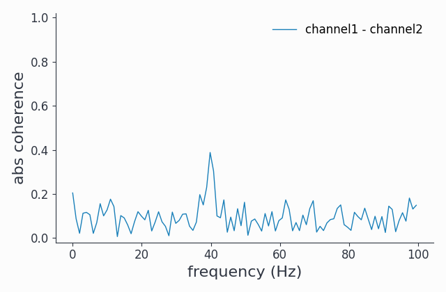
Indeed, we now see some coherence around the 40Hz band.

Finally, let’s wipe the inplace selection before continuing:

# inspect active inplace selection
adata.selection
>>> Syncopy AnalogData selector with all channels, 201 times, 100 trials

# wipe selection
adata.selection = None

Inplace selection via select keyword

Alternatively, we can also give a dictionary of selection parameters directly to every Syncopy meta-function. These will then internally apply an inplace selection before performing the analysis:

# coherence only for selected time points
coh3 = spy.connectivityanalysis(adata, method='coh', select={'latency': [-1, 0]})

# plot coherence of channel1 vs channel2
coh3.singlepanelplot(channel_i='channel1', channel_j='channel2')

Hopefully not surprisingly we get to exactly the same result as with an explicit in-place selection above. The difference here however is, that after the analysis is done, there is no active in-place selection present:

adata.selection is None
>>> True

Hence, it’s important to note that implicit selections get wiped automatically after an analysis.

In the end it is up to the user to decide which way of applying selections is most practical in their situation.

Relation to show() and singlepanelplot()

As hinted on in the beginning of this chapter, both plotting and numpy array extraction adhere to the same syntax as selectdata(). Meaning that the following two arrays hold the same data:

# First explicitly select a subset
trial10 = spy.selectdata(AData, trials=10, channel=["channel02", "channel06"])
# show everything of the subset
# WARNING: don't do this with large datasets!
arr1 = trial10.show()

# calling show() with the same selection
# criteria directly on the original complete dataset
arr2 = AData.show(trials=10, channel=["channel02", "channel06"])

# this is True!
arr1 == arr2

And in the same spirit, both plotting commands below will produce the same figure:

# First explicitly select a subset
trial10 = spy.selectdata(AData, trials=10, channel=["channel02", "channel06"])
# plot everything: only 1 trial and 2 channels left
trial10.singlepanelplot()

# directly plot from full data set with same selection criteria
AData.singlepanelplot(trials=10, channel=["channel02", "channel06"])

This works under the hood by applying temporary in-place selections onto the data before plotting and/or extracting the numpy arrays.