Syncopy for FieldTrip Users#
Syncopy is written in the Python programming language using the NumPy and SciPy libraries for computing as well as Dask for parallelization. The scope of Syncopy is limited to emulate parts of FieldTrip, in particular spectral and connectivity analysis of electrophysiology data. However, its call signatures and parameter names are designed to mimic the MATLAB analysis toolbox FieldTrip.
Note
MEGM/EEG-specific routines such as loading M/EEG file types, source localization, etc. are currently not included in Syncopy. For a Python toolbox tailored to MEG/EEG data analysis, see for example the MNE Project.
Exchanging Data between FieldTrip and Syncopy#
MAT-Files can be imported directly into Syncopy via load_ft_raw(), at the moment only the ft_datatype_raw is supported:
|
Imports raw time-series data from Field Trip into potentially multiple |
Key Differences between Syncopy and FieldTrip#
Have a look at the Quickstart with Syncopy page to quickly walk through a few Syncopy examples.
Installation and Setup#
Matlab comes as an all in one software package, and additional components like FieldTrip can be added as toolboxes within the Matlab desktop program.
Syncopy relies on the scientific Python ecosystem, a vast collection of open source programs and tools:
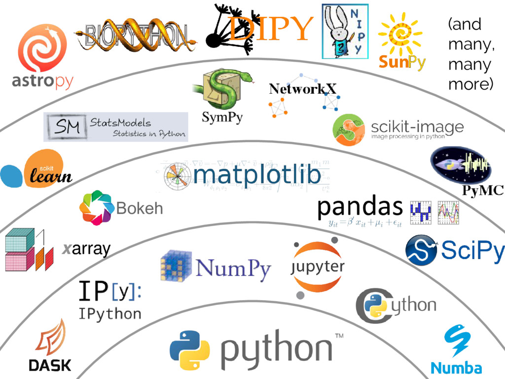
Source: VanderPlas 2017, slide 52.#
Managing Python environments and installing packages can be a challenging topic. The Anaconda Distribution eases a lot of those pains for new Python users, and is very popular within the scientific Python community. It also comes with the graphical Anaconda Navigator, which allows easy installation and execution of scientific Python programs like Jupyter or IPython console. Syncopy itself can be installed via anaconda, see Install Syncopy for details.
Interpreter and IDE#
Matlab as a commercial software is a bundle consisting of the Matlab interpreter and the IDE. Both are integrated into a single program with a user interface (UI), the Matlab desktop application.
Note
An interpreter is the place to interactively run commands (like randn(10, 2) in Matlab), and an IDE (integrated development environment) is the editor where scripts or programs are written.
Conversely, within the open source Python ecosystem there exists no inherent coupling between the IDE and the interpreter. So there is no universal Python desktop program but a variety of different possible setups. Three common solutions for scientific Python development are:
interactive computing in the browser
bundles scripting (IDE) and code execution (interpreter)
easy to set up, recommended for Python beginners
Editor + IPython console
keeps IDE and interpreter separate
free choice of popular editors like VS Code or Sublime Text
recommended for people with programming experience
tries to mimick the Matlab environment
integrates IDE and interpreter into a single desktop app
not very widespread but probably the most user friendly
Data types and handling#
The data in Syncopy is represented as Python objects. So it has methods (functions) and attributes (data) attached, accessible via the . operator. Let’s have a look at an AnalogData example:
import syncopy as spy

# red noise AR(1) process with 10 trials and 250 samples
adata = spy.synthdata.red_noise(alpha=0.9, nTrials=10, nSamples=250)

# access the filename attribute
adata.filename
this will print something like:
/path/to/.spy/tmp_storage/spy_fe2c_493b3197.analog
For an overview over all attributes of a specific Syncopy data object just type its name directly into your interpreter:
>>> adata

 Syncopy AnalogData object with fields

          cfg : dictionary with keys ''
      channel : [2] element <class 'numpy.ndarray'>
    container : None
         data : 10 trials of length 250.0 defined on [2500 x 2] float32 Dataset of size 0.02 MB
       dimord : time by channel
     filename : /xxx/xxx/.spy/spy_910e_572582c9.analog
         mode : r+
   sampleinfo : [10 x 2] element <class 'numpy.ndarray'>
   samplerate : 1000.0
          tag : None
         time : 10 element iterable
    trialinfo : [50 x 0] element <class 'numpy.ndarray'>
       trials : 10 element iterable

 Use `.log` to see object history
Hint
This works with Pythons neat string representation of classes. Try typing the name of a string variable (var = 'some string') into your interpreter.
Every Syncopy data object has the following attributes:
trials: returns a single trial asnumpy.ndarrayor an iterablechannel: stringnumpy.ndarrayof channel labelstrialdefinition:numpy.ndarrayrepresenting start, stop and offset off each trialsamplerate: the samplerate in Hzfilename: the path to the data file on discdata: the backing hdf5 dataset. You should not need to interact with this directly.
Each data class can have special attributes, for example freq for SpectralData. An extensive overview over all data classes can be found here: Syncopy Data Classes.
Functions and methods operating on data, like I/O and plotting can be found at Syncopy Data Basics.
Changing Attributes#
The attributes of Syncopy data objects typically mirror the fields of MatLab structures, however they cannot be simply overwritten:
adata.channel = 3
this gives:
SPYTypeError: Wrong type of `channel`: expected array_like found int
Syncopy has detailed error handling, and tries to tell you what exactly is wrong. So here, an array_like was expected, but a single int was the input. array_like basically means a sequence type, so numpy.ndarray or Python list. Let’s try again:
adata.channel = ['c1', 'c2', 'c3']
Still no good:
SPYValueError: Invalid value of `channel`: 'shape = (3,)'; expected array of shape (2,)
So in NumPy language that tells us, that Syncopy expected an array with two elements instead of three. Inspecting the channel attribute:
adata.channel
array(['channel1', 'channel2'], dtype='<U8')
we see that we have only two channels in this case, so setting three channel labels indeed makes no sense. Finally with:
adata.channel = ['c1', 'c2']
we can change the channel labels.
Translating MATLAB Code to Python#
For translating code from MATLAB to Python there are several guides, e.g.
Key Differences between the Python and MATLAB Languages#
While the above links cover differences between Python and MATLAB to a great extent, we highlight here what we think are the most important differences:
Indexing is different - Python array indexing starts at 0:
>>> x = [1, 2, 3, 4]
>>> x[0]
1
Python ranges are half-open intervals
[left, right), i.e., the right boundary is not included:>>> list(range(1, 4)) [1, 2, 3]
Data in Python is not necessarily copied and may be manipulated in-place:
>>> x = [1, 2, 3, 4]
>>> y = x
>>> x[0] = -1
>>> y
[-1, 2, 3, 4]
To prevent this an explicit copy of a list, numpy.array, etc. can be requested:
>>> x = [1, 2,3 ,4]
>>> y = list(x)
>>> x[0] = -1
>>> y
[1, 2, 3, 4]
Python’s powerful import system allows simple function names (e.g.,
load()) without worrying about overwriting built-in functions>>> import syncopy as spy >>> import numpy as np >>> spy.load <function syncopy.io.load_spy_container.load(filename, tag=None, dataclass=None, checksum=False, mode='r+', out=None) >>> np.load <function numpy.load(file, mmap_mode=None, allow_pickle=False, fix_imports=True, encoding='ASCII')>
Project-specific environments allow reproducible and customizable work setups.
$ conda activate np17
$ python -c "import numpy; print(numpy.version.version)"
1.17.2
$ conda activate np15
$ python -c "import numpy; print(numpy.version.version)"
1.15.4
Translating FieldTrip Calls to Syncopy#
Using a FieldTrip function in MATLAB usually works via constructing a cfg
struct that contains all necessary configuration parameters:
ft_defaults
cfg = [];
cfg.option1 = 'yes';
cfg.option2 = [10, 20];
result = ft_something(cfg);
Syncopy emulates this concept using a syncopy.StructDict (really just a
slightly modified Python dictionary) that can automatically be filled with
default settings of any function.
import syncopy as spy
cfg = spy.get_defaults(spy.something)
cfg.option1 = 'yes'
# or
cfg.option1 = True
cfg.option2 = [10, 20]
result = spy.something(cfg)
A FieldTrip Power Spectrum in Syncopy#
For example, a power spectrum calculated with FieldTrip via
cfg = [];
cfg.method = 'mtmfft';
cfg.foilim = [1 150];
cfg.output = 'pow';
cfg.taper = 'dpss';
cfg.tapsmofrq = 10;
spec = ft_freqanalysis(cfg, data)
can be computed in Syncopy with
cfg = spy.get_defaults(spy.freqanalysis)
cfg.method = 'mtmfft'
cfg.foilim = [1, 150]
cfg.output = 'pow'
cfg.tapsmofrq = 10
spec = spy.freqanalysis(cfg, data)
Key Differences between FieldTrip and Syncopy#
FieldTrip has a lot more features. Syncopy is still in early development and will never cover the rich feature-set of FieldTrip.
FieldTrip supports many data formats. Syncopy currently only supports data import from FieldTrip (see below).
Syncopy data objects use disk-streaming and are thus never fully loaded into memory.
Experimental import/export from MatLab#
See Roundtrip from MatLab - FieldTrip to Syncopy and Back for an example.