Preprocessing

Raw data often contains unwanted signal components: offsets, trends or even oscillatory nuisance signals. Syncopy has a dedicated preprocessing() function to clean up and/or transform the data.

Let’s start by creating a new synthetic signal with confounding components:

# built-in synthetic data generators
import syncopy as spy
from syncopy import synthdata as spy_synth

cfg_synth = spy.StructDict()
cfg_synth.nTrials = 150
cfg_synth.samplerate = 500
cfg_synth.nSamples = 1000
cfg_synth.nChannels = 2

# 30Hz undamped harmonig
harm = spy_synth.harmonic(cfg_synth, freq=30)

# a linear trend
lin_trend = spy_synth.linear_trend(cfg_synth, y_max=3)

# a 2nd 'nuisance' harmonic
harm50 = spy_synth.harmonic(cfg_synth, freq=50)

# finally the white noise floor
wn = spy_synth.white_noise(cfg_synth)

Here we used a cfg dictionary to assemble all needed parameters, a concept we adopted from FieldTrip

Dataset Arithmetics

If the shape of different Syncopy objects match exactly (nSamples, nChannels and nTrials are all the same), we can use standard Python arithmetic operators like +, -, * and / directly. Here we want a linear superposition, so we simply add everything together:

# add noise, trend and the nuisance harmonic
data_nui = harm + wn + lin_trend + harm50
# also works for scalars
data_nui = data_nui + 5

If we now do a spectral analysis, the power spectra are confounded by all our new signal components:

cfg = spy.StructDict()
cfg.tapsmofrq = 1
cfg.foilim = [0, 60]
cfg.polyremoval = None
cfg.keeptrials = False   # trial averaging
fft_nui_spectra = spy.freqanalysis(data_nui, cfg)

Note

We explicitly set polyremoval=None to see the full effect of our confounding signal components. The default for freqanalysis() is polyremoval=0, which removes polynoms of 0th order: constant offsets (de-meaning).

Hint

We did not specify the method parameter for the freqanalysis() call as multi-tapered Fourier analysis (method='mtmfft') is the default. To learn about the defaults of any Python function you can inspect its signature with spy.freqanalysis? or help(spy.freqanalysis) typed into an interpreter

Let’s see what we got:

fft_nui_spectra.singlepanelplot()

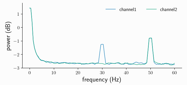
We see strong low-frequency components, originating from both the offset and the trend. We also see the nuisance signal spectral peak at 50Hz.

Filtering

Filtering of signals in general removes/suppresses unwanted signal components. This can be done both in the time-domain and in the frequency-domain. For offsets and (low-order) polynomial trends, fitting a model directly in the time domain, and subtracting the obtained trend, is the preferred solution. This can be controlled in Syncopy with the polyremoval parameter, which is also directly available in freqanalysis().

Removing signal components in the frequency domain is typically done with finite impulse response (FIR) filters or infinite impulse response (IIR) filters. Syncopy supports one of each kind, a FIR windowed sinc and the Butterworth filter from the IIR family. For both filters we have low-pass ('lp'), high-pass ('hp'), band-pass ('bp') and band-stop(Notch) ('bp') designs available.

To clean up our dataset above, we remove the linear trend and apply a low-pass 12th order Butterworth filter:

data_pp = spy.preprocessing(data_nui,
                            filter_class='but',
                            filter_type='lp',
                            polyremoval=1,
                            freq=40,
                            order=12)

Now let’s reuse our cfg from above to repeat the spectral analysis with the preprocessed data:

spec_pp = spy.freqanalysis(data_pp, cfg)
spec_pp.singlepanelplot()

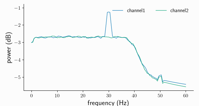
As expected for a low-pass filter, all frequencies above 40Hz are strongly attenuated (note the log scale, so the suppression is around 2 orders of magnitude). We also removed the low-frequency components from the offset and trend, but acknowledge that we also lost a bit of the original white noise power around 0-2Hz. Importantly, the spectral power of our frequency band of interest, around 30Hz, remained virtually unchanged.