Using FOOOF from Syncopy

Syncopy supports parameterization of neural power spectra using the Fitting oscillations & one over f (FOOOF ) method described in the following publication (DOI link):

Donoghue T, Haller M, Peterson EJ, Varma P, Sebastian P, Gao R, Noto T, Lara AH, Wallis JD, Knight RT, Shestyuk A, & Voytek B (2020). Parameterizing neural power spectra into periodic and aperiodic components. Nature Neuroscience, 23, 1655-1665. DOI: 10.1038/s41593-020-00744-x

The FOOOF method requires as input an Syncopy AnalogData object, so time series data like an LFP signal. Applying FOOOF can then be seen as a post-processing of a multi-tapered Fourier Analysis.

Generating Example Data

Let us first prepare suitable data. FOOOF will typically be applied to trial-averaged data, as the method is quite sensitive to noise, so we generate an example data set consisting of 500 trials and a single channel here (see Synthetic data tutorial for details on this):

import numpy as np
import syncopy as spy
from syncopy.synthdata import red_noise, phase_diffusion

def create_trials(nTrials = 500):

    cfg_synth = spy.StructDict()
    cfg_synth.nSamples = 1000
    cfg_synth.samplerate = 1000
    cfg_synth.nChannels = 1
    cfg_synth.nTrials = nTrials

    ar1_traj = red_noise(cfg_synth, alpha=0.9)
    pd1 = phase_diffusion(cfg_synth, freq=30., eps=.1)
    pd2 = phase_diffusion(cfg_synth, freq=50., eps=.1)

    # add weighted signal components together
    signal = ar1_traj + .8 * pd1 + 0.6 * pd2
    return signal

signals = create_trials()

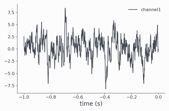
The return value signals is of type AnalogData. Let’s have a look at the signal in the time domain first:

signals.singlepanelplot(trials = 0)

Since FOOOF works on the power spectrum, we can perform an mtmfft and look at the results to get a better idea of how our data looks in the (un-fooofed) frequency domain. The spec data structure we obtain is of type SpectralData, and can also be plotted:

cfg = spy.StructDict()
cfg.method = "mtmfft"
cfg.taper = "hann"
# cfg.select = {"channel": 0}
cfg.keeptrials = False
cfg.output = "pow"
cfg.foilim = [10, 100]

spec = spy.freqanalysis(cfg, signals)
spec.singlepanelplot()

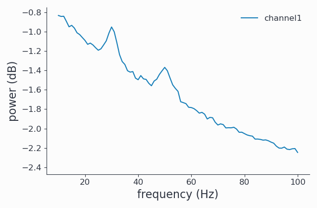
By construction, we see two spectral peaks around 30Hz and 50Hz and a strong \(1/f\) like background.

Running FOOOF

Now that we have seen the more or less raw power spectrum, let us start FOOOF. The FOOOF method is accessible from the freqanalysis function by setting the output parameter to ‘fooof’:

cfg.output = 'fooof'
spec_fooof = spy.freqanalysis(cfg, signals)
spec_fooof.singlepanelplot()

FOOOF output types

In the example above, the spectrum returned is the full FOOOFed spectrum. This is typically what you want, but to better understand your results, you may be interested in the other options. The following ouput types are available:

• fooof: the full fooofed spectrum

• fooo_aperiodic: the aperiodic part of the spectrum

• fooof_peaks: the detected peaks, with Gaussian fit to them

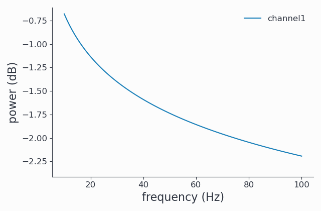
Here we request only the aperiodic (\(\sim 1/f\)) part and plot it:

cfg.output = 'fooof_aperiodic'
spec_fooof_aperiodic = spy.freqanalysis(cfg, signals)
spec_fooof_aperiodic.singlepanelplot()

You may want to use a combination of the different return types to inspect your results.

Knowing what your data and the FOOOF results like is important, because typically you will have to fine-tune the FOOOF method to get the results you are interested in.

With the data above, we were interested only in the 2 large peaks around 30 and 50 Hz, but 2 more minor peaks were detected by FOOOF, around 37 and 42 Hz. We will learn how to exclude these peaks in the next section.

Fine-tuning FOOOF

The FOOOF method can be adjusted using the fooof_opt parameter to freqanalyis. The full list of available options and defaults are explained in detail in the official FOOOF documentation.

From the results above, we see that some peaks were detected that we think (and actually know by construction) are noise. Increasing the minimal peak width is one method to exclude them:

cfg.output = 'fooof'
cfg.fooof_opt = {'peak_width_limits': (6.0, 12.0), 'min_peak_height': 0.2}
spec_fooof_tuned = spy.freqanalysis(cfg, signals)
spec_fooof_tuned.singlepanelplot()

Once more, we look at the FOOOFed spectrum:

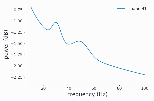
Note that the two tiny peaks have been removed.

Programmatically accessing details on the FOOOF fit results

All fitting results returned by FOOOF can be found in the metadata attribute of the returned SpectralData instance, which is a dict. This includes the following entries:

• aperiodic_params (offset, exponent)

• peak_params (center frequency, power above aperiodic, bandwidth)

• gaussian_params (mean, height, standard deviation) of the peaks

• n_peaks (number of peaks)

• r_squared (goodness of fit)

• error (RMSE)

Please see the official FOOOF documentation for the meaning.

Note that in Syncopy, FOOOF can be run several times in a single frontend call, e.i. you work with single trial spectra and keep the default cfg.keeptrials=True. Therefore, you will see one instance of these fitting results per trial (that is per FOOOF call) in the metadata dict. The trials (and chunk indices, if you used a non-default chan_per_worker setting) are encoded in the keys of the metadata sub dictionaries in format <result>__<trial>_<chunk>. E.g., peak_params__2__0 would be the peak params for trial 2 (and chunk 0).

In the example above, the typical use case of trial averaging (cfg.keeptrials=False) was demonstrated, so FOOOF operated on the trial-averaged spectrum (i.e., on effectively a single trial), and only one entry is present:

spec_fooof_tuned.metadata
# {'aperiodic_params': {'aperiodic_params__0_0': array([[0.8006], [1.4998]])},
# ...

This concludes the tutorial on using FOOOF from Syncopy. Please do not forget to cite Donoghue et al. 2020 when using FOOOF.